 Korean
 English
: Baby steps to your neural network's first memories.
* This is the Korean translation of the original post by @iamtrask under his permission. You can find the English version at his blog: here. 저자의 허락을 득하고 번역하여 옮깁니다.
# 여기 나오는 예제에 제가 조금 더 내용을 추가한 것을 ipynb으로 만들어 정리해보았습니다.
* github 링크: https://github.com/jaejun-yoo/RNN-implementation-using-Numpy-binary-digit-addition
* blog 링크: https://jaejunyoo.blogspot.com/2017/06/rnn-implementation-using-only-numpy.html
* github 링크: https://github.com/jaejun-yoo/RNN-implementation-using-Numpy-binary-digit-addition
* blog 링크: https://jaejunyoo.blogspot.com/2017/06/rnn-implementation-using-only-numpy.html
요약: 저는 제가 다루기 쉬운 toy code를 가지고 놀 때 가장 잘 배우는 것 같습니다. 이 튜토리얼은 매우 쉬운 예제와 짧은 파이썬 코드를 바탕으로 Recurrent Neural Networks (RNN)에 대해 설명을 진행합니다.
(원작자: Part2: LSTM에 대해서는 작성이 완료되는대로 @iamtrask에 트윗할 것이니 팔로우 해주세요. 어떤 피드백이든 환영입니다.)
Just Give Me The Code:
001.import copy, numpy as np002.np.random.seed(0)003. 004.# compute sigmoid nonlinearity005.def sigmoid(x):006.output = 1/(1+np.exp(-x))007.return output008. 009.# convert output of sigmoid function to its derivative010.def sigmoid_output_to_derivative(output):011.return output*(1-output)012. 013. 014.# training dataset generation015.int2binary = {}016.binary_dim = 8017. 018.largest_number = pow(2,binary_dim)019.binary = np.unpackbits(020.np.array([range(largest_number)],dtype=np.uint8).T,axis=1)021.for i in range(largest_number):022.int2binary[i] = binary[i]023. 024. 025.# input variables026.alpha = 0.1027.input_dim = 2028.hidden_dim = 16029.output_dim = 1030. 031. 032.# initialize neural network weights033.synapse_0 = 2*np.random.random((input_dim,hidden_dim)) - 1034.synapse_1 = 2*np.random.random((hidden_dim,output_dim)) - 1035.synapse_h = 2*np.random.random((hidden_dim,hidden_dim)) - 1036. 037.synapse_0_update = np.zeros_like(synapse_0)038.synapse_1_update = np.zeros_like(synapse_1)039.synapse_h_update = np.zeros_like(synapse_h)040. 041.# training logic042.for j in range(10000):043. 044.# generate a simple addition problem (a + b = c)045.a_int = np.random.randint(largest_number/2) # int version046.a = int2binary[a_int] # binary encoding047. 048.b_int = np.random.randint(largest_number/2) # int version049.b = int2binary[b_int] # binary encoding050. 051.# true answer052.c_int = a_int + b_int053.c = int2binary[c_int]054. 055.# where we'll store our best guess (binary encoded)056.d = np.zeros_like(c)057. 058.overallError = 0059. 060.layer_2_deltas = list()061.layer_1_values = list()062.layer_1_values.append(np.zeros(hidden_dim))063. 064.# moving along the positions in the binary encoding065.for position in range(binary_dim):066. 067.# generate input and output068.X = np.array([[a[binary_dim - position - 1],b[binary_dim -position - 1]]])069.y = np.array([[c[binary_dim - position - 1]]]).T070. 071.# hidden layer (input ~+ prev_hidden)072.layer_1 = sigmoid(np.dot(X,synapse_0) +np.dot(layer_1_values[-1],synapse_h))073. 074.# output layer (new binary representation)075.layer_2 = sigmoid(np.dot(layer_1,synapse_1))076. 077.# did we miss?... if so, by how much?078.layer_2_error = y - layer_2079.layer_2_deltas.append((layer_2_error)*sigmoid_output_to_derivative(layer_2))080.overallError += np.abs(layer_2_error[0])081. 082.# decode estimate so we can print it out083.d[binary_dim - position - 1] = np.round(layer_2[0][0])084. 085.# store hidden layer so we can use it in the next timestep086.layer_1_values.append(copy.deepcopy(layer_1))087. 088.future_layer_1_delta = np.zeros(hidden_dim)089. 090.for position in range(binary_dim):091. 092.X = np.array([[a[position],b[position]]])093.layer_1 = layer_1_values[-position-1]094.prev_layer_1 = layer_1_values[-position-2]095. 096.# error at output layer097.layer_2_delta = layer_2_deltas[-position-1]098.# error at hidden layer099.layer_1_delta = (future_layer_1_delta.dot(synapse_h.T) +layer_2_delta.dot(synapse_1.T)) *sigmoid_output_to_derivative(layer_1)100. 101.# let's update all our weights so we can try again102.synapse_1_update +=np.atleast_2d(layer_1).T.dot(layer_2_delta)103.synapse_h_update +=np.atleast_2d(prev_layer_1).T.dot(layer_1_delta)104.synapse_0_update += X.T.dot(layer_1_delta)105. 106.future_layer_1_delta = layer_1_delta107. 108. 109.synapse_0 += synapse_0_update * alpha110.synapse_1 += synapse_1_update * alpha111.synapse_h += synapse_h_update * alpha 112. 113.synapse_0_update *= 0114.synapse_1_update *= 0115.synapse_h_update *= 0116. 117.# print out progress118.if(j % 1000 == 0):119.print "Error:" + str(overallError)120.print "Pred:" + str(d)121.print "True:" + str(c)122.out = 0123.for index,x in enumerate(reversed(d)):124.out += x*pow(2,index)125.print str(a_int) + " + " + str(b_int) + " = " + str(out)126.print "------------"127. 128.Runtime Output:
Error:[ 3.45638663]
Pred:[0 0 0 0 0 0 0 1]
True:[0 1 0 0 0 1 0 1]
9 + 60 = 1
------------
Error:[ 3.63389116]
Pred:[1 1 1 1 1 1 1 1]
True:[0 0 1 1 1 1 1 1]
28 + 35 = 255
------------
Error:[ 3.91366595]
Pred:[0 1 0 0 1 0 0 0]
True:[1 0 1 0 0 0 0 0]
116 + 44 = 72
------------
Error:[ 3.72191702]
Pred:[1 1 0 1 1 1 1 1]
True:[0 1 0 0 1 1 0 1]
4 + 73 = 223
------------
Error:[ 3.5852713]
Pred:[0 0 0 0 1 0 0 0]
True:[0 1 0 1 0 0 1 0]
71 + 11 = 8
------------
Error:[ 2.53352328]
Pred:[1 0 1 0 0 0 1 0]
True:[1 1 0 0 0 0 1 0]
81 + 113 = 162
------------
Error:[ 0.57691441]
Pred:[0 1 0 1 0 0 0 1]
True:[0 1 0 1 0 0 0 1]
81 + 0 = 81
------------
Error:[ 1.42589952]
Pred:[1 0 0 0 0 0 0 1]
True:[1 0 0 0 0 0 0 1]
4 + 125 = 129
------------
Error:[ 0.47477457]
Pred:[0 0 1 1 1 0 0 0]
True:[0 0 1 1 1 0 0 0]
39 + 17 = 56
------------
Error:[ 0.21595037]
Pred:[0 0 0 0 1 1 1 0]
True:[0 0 0 0 1 1 1 0]
11 + 3 = 14
------------
Part 1: Neural Memory란?
알파벳을 순서대로 읊어보세요...쉽게 할 수 있죠? 그럼 이번엔 알파벳을 거꾸로 읊어보려 해보세요...흠....아마 이건 조금 더 어려울 것입니다.
잘 아는 노래 가사에 똑같이 시도해보세요. 왜 순서대로 떠올리는 것이 거꾸로 떠올리는 것보다 쉬울까요? 혹시 2절의 중간 부분으로 뛰어넘어 부를 수 있나요...흠...이것도 쉽진 않죠? 왜 그럴까요?
여기에는 아주 논리적인 근거가 있습니다. 인간은 알파벳이나 노래 가사를 컴퓨터처럼 하드 드라이브에 저장하는 것이 아니기 때문에 그렇습니다. 인간은 이런 정보를 하나의 sequence로 학습합니다. 이전 알파벳에서 다음으로 넘어가는 것은 매우 잘 하는 것을 볼 수 있고 이런 것은 조건부 기억이라 할 수 있습니다. 즉, 최근에 바로 이전 기억이 있을 때만 기억을 불러 올 수 있는 것이죠. 어찌보면 linked list(만약 이 개념이 익숙하시다면)와 유사한 점이 많습니다.
그렇다고 해서 당신이 그 노래를 부를 때 외에는 기억하지 못하는 것은 아니죠. 다만 갑자기 바로 중간부터 노래를 부르려하면 당신의 뇌에서 (아마도 뉴런들 한 뭉치가) 적절한 위치를 찾아내는데 약간 시간이 걸릴뿐입니다. 노래의 중간 부분 가사를 찾기 위해 처음부터 쭉 다시 되짚는데 이게 딱히 전에 이런 식으로 찾으려 시도한 적이 없었기 때문에 뇌에서 이 정보가 위치하는 곳으로 이어지는 어떤 지도가 딱 있지 않아 그렇습니다.
비유하자면 막다른 골목이나 후미진 곳이 많은 동네에서 사는 것과 비슷합니다. 길을 이용해서 동네를 많이 다녀봤기 때문에 어떤 사람의 집으로 가는 방법을 길을 따라 상상하는 것은 쉽지만 다니던 길이 아닌 직선으로 어떤 사람의 뒷마당을 가로질러 가는 법을 생각하는 것은 쉽지 않죠. 그러니까 인간의 뇌는 "방향"을 사용해서 정보를 기억하고, 노래와 같은 경우 그 첫 부분을 기억하는 뉴런에서부터 시작해서 하나씩 되짚어 갑니다. (for more on brain stuff, click here)
마치 linked list처럼 이런 방식으로 기억을 저장하는 것은 매우 효율적입니다. 마찬가지로 기억이라는 요소를 뉴럴 네트워크에 추가하는 것이 이와 비슷한 장점이 있다는 것을 소개하겠습니다. 특히 어떤 프로세스나 문제들의 경우, 이렇게 단기 기억 혹은 유사 조건부 메모리를 이용한 sequence로 모델링을 하는 것이 매우 효율적일 때가 있습니다.
기억이란 것은 데이터가 어떤 형태의 sequence일 때 매우 중요합니다. (이는 뭔가 기억할 것이 있다는 말이죠!) 가령 우리 데이터가 아래와 같이 통통 튀는 공을 찍은 영상이라 해보겠습니다.
이 경우, 비디오의 각 프레임이 하나의 데이터가 됩니다. 뉴럴 네트워크를 학습시켜서 다음 프레임에 공이 어디에 있을지 예측하도록 하고 싶다면 그 전 프레임에서 공이 어디에 있었는지를 아는 것이 매우 도움이 되겠죠. 이런 연속적인 데이터를 다루기 위해 RNN을 사용합니다. 그럼 뉴럴 네트워크가 이전 시간 단계(time step)에서 무엇을 봤는지 어떻게 기억할까요?
뉴럴 네트워크에는 hidden layers가 있습니다. 보통 이런 hidden layer는 input data에만 의존하지요. 그래서 일반적인 뉴럴 네트워크의 정보 흐름을 보면 다음과 같습니다:
뉴럴 네트워크에는 hidden layers가 있습니다. 보통 이런 hidden layer는 input data에만 의존하지요. 그래서 일반적인 뉴럴 네트워크의 정보 흐름을 보면 다음과 같습니다:
input -> hidden -> output
이건 매우 직관적이죠. 특정 형태의 input은 hidden layer의 형태를 결정하고 이에 따라 output layer의 타입도 결정됩니다. 메모리라는 개념이 들어가면 이 구조가 바뀝니다. 메모리가 있다는 것은 hidden layer가 현재 단계의 input data와 이전 단계의 hidden layer의 조합으로 이루어진다는 것을 의미합니다.
(input + prev_hidden)->hidden->output
왜 하필 hidden layer일까요? 물론 아래와 같이 할 수도 있습니다.
(input + prev_input)->hidden->output
하지만, 이렇게 할 경우 뭔가 놓치는 것이 생깁니다. 잠시 앉아서 앞서 소개한 정보의 흐름이 어떤 차이가 있을지 고민해보시길 권합니다. 약간 힌트를 드리자면, 어떤 식으로 움직이는지 살펴보시는 것이 좋습니다. 자, 다음과 같이 4 timesteps of RNN pulling 정보가 이전 hidden layer로부터 왔다고 해봅시다:
(input + empty_hidden) -> hidden -> output
(input + prev_hidden) -> hidden -> output
(input + prev_hidden) -> hidden -> output
(input + prev_hidden) -> hidden -> output
그리고 이와는 다르게 hidden layer가 아니라 previous input layer로부터 정보가 들어오면 다음과 같이 나타낼 수 있습니다:
약간 더 이해를 돕기 위해 각각의 경우에 대해 색을 칠해보겠습니다:
hidden layer recurrence:
(input + empty_hidden) -> hidden -> output
(input + prev_hidden) -> hidden -> output
(input + prev_hidden) -> hidden -> output
(input + prev_hidden ) -> hidden -> output
.... and 4 timesteps with input layer recurrence....
(input + empty_input) -> hidden -> output
(input + prev_input) -> hidden -> output
(input + prev_input) -> hidden -> output
(input + prev_input) -> hidden -> output
(input + empty_input) -> hidden -> output
(input + prev_input) -> hidden -> output
(input + prev_input) -> hidden -> output
(input + prev_input) -> hidden -> output
약간 더 이해를 돕기 위해 각각의 경우에 대해 색을 칠해보겠습니다:
hidden layer recurrence:
.... and 4 timesteps with input layer recurrence....
마지막 hidden layer(4th line)을 주목해주세요. Hidden layer recurrence를 보시면 지금까지 본 모든 input이 존재하는 것을 볼 수 있습니다. 반면에 input layer recurrence의 경우 현재와 바로 직전 input에 대해서만 정의 되는 것을 보실 수 있습니다 (* 역자 주: 색깔의 종류 수를 보세요). Hidden recurrence는 어떤 것을 기억할지를 학습하는 반면에 input recurrence는 바로 직전 데이터를 외우도록 고정이 된 (hard wired) 것을 보실 수 있습다.
이제 이 두 가지 방식을 알파벳 거꾸로 떠올리기 그리고 중간 가사부터 노래 부르기에 적용하여 비교해보겠습니다. Hidden layer는 inputs을 받을 때마다 계속 바뀝니다. 게다가 우리가 이런 hidden states에 도달할 방법은 입력이 올바른 순서(sequence)로 있을 때뿐입니다.
이제 이 두 가지 방식을 알파벳 거꾸로 떠올리기 그리고 중간 가사부터 노래 부르기에 적용하여 비교해보겠습니다. Hidden layer는 inputs을 받을 때마다 계속 바뀝니다. 게다가 우리가 이런 hidden states에 도달할 방법은 입력이 올바른 순서(sequence)로 있을 때뿐입니다.
우리가 노래 가사의 이전 부분을 알 때 다음 단어를 예측하려 한다고 해봅시다. "Input layer recurrence" 방식의 경우 노래에 우연히도 같은 sequence가 여러 위치에 나올 경우 문제가 생깁니다. 노래에 "I love you"와 "I love carrots"라는 가사가 들어간다고 해봅시다. 그리고 네트워크가 다음 단어를 에측하려고 한다면 "I love" 다음에 뭐가 올지 어떻게 예측할까요? 분명 답은 carrot일 수도 있고 you일 수도 있습니다만 제대로 예측을 하려면 현재 노래가 전체에서 어떤 부분이 지나가고 있는지를 알아야만 합니다. "Hidden layer recurrence"의 경우 바로 이전 정보만을 가지고 있는 것이 아니라 지금까지 본 것을 어떤 식으로든 기억하고 있기 때문에 (물론 현재 단계로부터 먼 과거의 정보로 갈수록 점점 기억이 희미하게 남아있겠지만) 문제가 생기지 않습니다. To see this in action, check out this.
잠시 멈춰서 지금까지 얘기한 내용이 당연하게 느껴질 때까지 시간을 갖고 고민해보세요.
Part 2: RNN - Neural Network Memory
이제 아이디어는 알았으니 좀 더 구체적으로 가봅시다. 앞서 얘기하였듯 메모리라는 것은 hidden layer가 input data와 이전 hidden layer의 조합으로 만들어진다는 것을 뜻합니다. 이걸 어떻게 하면 될까요? 다른 뉴럴 네트워크의 propagation과 같이 행렬의 형태로 표현할 수 있습니다.
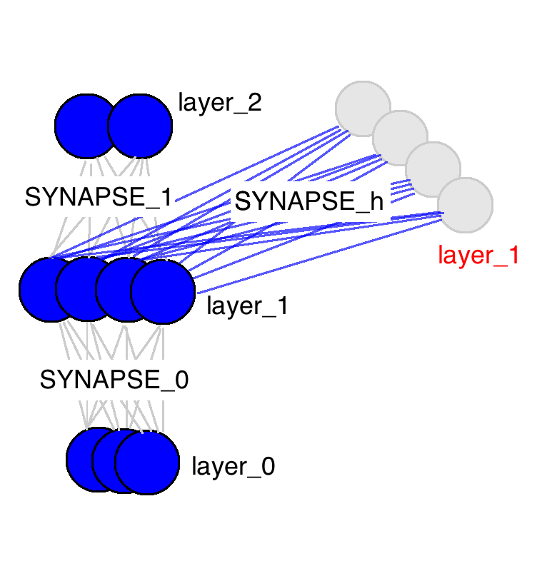
위 그림의 뉴럴 네트워크는 weight 행렬이 딱 세 개 있습니다. 두 개는 익숙하지요? input layer인 layer_0와 hidden layer인 layer_1을 잇는 SYNAPSE_0와 hidden layer에서 output으로 이어지는 SYNAPSE_1이 있습니다. 여기에 새로운 행렬이 하나 추가되는데요 SYNAPSE_h이 현재 hidden layer(layer_1)에서 다음 timestep(still layer_1)의 hidden layer로 반복(recurrent)하여 연산(propagate)이 됩니다.
stop and make sure this feels comfortable in your mind

이 gif가 RNN의 매우 매우 중요한 몇 가지 성질을 보여주고 있습니다. 네 개의 timestep이 있을 때, 첫번째는 input data에만 영향을 받습니다. 두번째에서는 새로 들어온 second input data와 이전 단계의 input data에 영향이 섞여 있습니다. 이런 식으로 네트워크가 4 timesteps이면 꽉 차는 것을 보실 수 있고 금새 예측하실 수 있듯이 5번째 timestep에서는 어떤 정보를 기억하고 어떤 것을 덮어씌울지 네트워크가 결정해야겠지요.
지금 이 그림은 단순히 예시가 아니라 실제로 RNN에서 일어나는 현상을 보여주고 있습니다. 이게 바로 네트워크의 기억 "용량"이 되는 것이지요. 당연히도 더 큰 layer가 더 오랜 기간에 대한 정보를 기억할 수 있습니다. 또한 네트워크가 관련 없어보이는 정보를 잊어버리고 중요한 정보를 기억하는 방법을 학습하는 것도 바로 이 때 일어나는 것이죠. (추가로 생각해볼 점: 3번째 단계에서 혹시 뭔가 특이한 점을 발견하셨나요? 왜 hidden layer에서 다른 색보다 녹색이 더 많을까요?)
이 외에도 hidden layer가 input과 output 사이의 barrier 역할을 한다는 사실을 확인하실 수 있습니다. 실제로, output이 더이상 순수히 input에 따라 바뀌는 함수가 아니며 input은 기억에 어떤 것이 들어갈 지를 바꿀뿐 output은 네트워크가 가지고 있는 기억에 따라 결정됩니다. Timestep 2,3,4에 아무런 input이 들어가지 않더라도 hidden layer는 매 timestep마다 바뀐다는 점도 짚고 넘어가시면 되겠습니다.
I know I've been stopping... but really make sure you got that last bit
Part 3: Backpropagation Through Time:
그럼 이제 RNN이 어떻게 학습을 하는지 배울 때가 왔습니다. 아래 그림을 확인해주세요. 검은색은 prediction, error는 밝은 노랑, derivatives는 머스터드 색입니다.

RNN은 1에서 4로 propagate하고 다시 4에서 1로 돌아오며 모든 derivatives를 backpropagate하는 것으로 학습을 합니다. 어떻게 보면 엄청 이상하게 생긴 일반적인 뉴럴 네트워크라고 생각하실 수도 있습니다. (weight, synapse 0,1, 그리고 h를 반복하여 사용한다는 점만 빼면) 이 부분을 제외하고는 일반적으로 우리가 알고 있는 backpropagation입니다.
Part 4: Our Toy Code
위 그림에서 색이 있는 박스 안에 들어가 있는 1들은 "carry bits"라고 합니다. 이 녀석들은 각 자릿수에서 더하고 넘치는 값을 들고 다니죠. 이 녀석들이 바로 우리 네트워크가 배워야할 아주 작은 메모리라고 할 수 있습니다.
(* 역자 주: 사실 이 그림에서 도무지 왜 저 이진수들이 각각 -1, -2, -3이 되는 것인지는 이해가 가지 않습니다만 -_-;; (<- 이 부분에 대해서 아래에 lili popo님이 답을 댓글로 주셨네요 음수를 2진법에서 나타내는 방식이 있는데 설명이 아래에 있으니 혹시 궁금하시면 확인하시면 되겠습니다.) 최소한 이진법에서 1과 1을 더했을 때 0이 나오고 다음 자리수로 1이 올라가는 형태란 것은 쉽게 유추할 수 있습니다. 여기서 얘기하고자 하는 것은 위의 그림과 같이 각각의 이진수의 자릿수 순서대로 sequence가 들어와서 더하기를 할 때 다음 자릿수에서 계산을 하려면 이전 자릿수에서 넘어온 overflow 1이 있는지 기억을 해야하므로 아주 작지만 메모리가 필요합니다. 이런 이진수 덧셈을 RNN으로 해보겠다는 것이죠.)
(여기서부터는 창을 하나 더 여셔서 맨 위의 code와 비교해가면서 글을 보시는 것이 편합니다. )
(* 역자 주: 이 부분이 상당히 크리티컬한 부분인데요 코드와 비교해가시면서 이해하시면 RNN에 대한 이해가 쉬이 되실 것 같습니다. 다만 코드 설명 부분까지 번역할 필요는 없어보여 원문을 그대로 두도록 하겠습니다. 혹시 요청이 있다면 하는 것으로..)
Lines 0-2: Importing our dependencies and seeding the random number generator. We will only use numpy and copy. Numpy is for matrix algebra. Copy is to copy things.
Lines 4-11: Our nonlinearity and derivative. For details, please read this Neural Network Tutorial
Line 15: We're going to create a lookup table that maps from an integer to its binary representation. The binary representations will be our input and output data for each math problem we try to get the network to solve. This lookup table will be very helpful in converting from integers to bit strings.
Line 16: This is where I set the maximum length of the binary numbers we'll be adding. If I've done everything right, you can adjust this to add potentially very large numbers.
Line 18: This computes the largest number that is possible to represent with the binary length we chose
Line 19: This is a lookup table that maps from an integer to its binary representation. We copy it into the int2binary. This is kindof un-ncessary but I thought it made things more obvious looking.
Line 26: This is our learning rate.
Line 27: We are adding two numbers together, so we'll be feeding in two-bit strings one character at the time each. Thus, we need to have two inputs to the network (one for each of the numbers being added).
Line 28: This is the size of the hidden layer that will be storing our carry bit. Notice that it is way larger than it theoretically needs to be. Play with this and see how it affects the speed of convergence. Do larger hidden dimensions make things train faster or slower? More iterations or fewer?
Line 29: Well, we're only predicting the sum, which is one number. Thus, we only need one output
Line 33: This is the matrix of weights that connects our input layer and our hidden layer. Thus, it has "input_dim" rows and "hidden_dim" columns. (2 x 16 unless you change it). If you forgot what it does, look for it in the pictures in Part 2 of this blogpost.
Line 34: This is the matrix of weights that connects the hidden layer to the output layer. Thus, it has "hidden_dim" rows and "output_dim" columns. (16 x 1 unless you change it). If you forgot what it does, look for it in the pictures in Part 2 of this blogpost.
Line 35: This is the matrix of weights that connects the hidden layer in the previous time-step to the hidden layer in the current timestep. It also connects the hidden layer in the current timestep to the hidden layer in the next timestep (we keep using it). Thus, it has the dimensionality of "hidden_dim" rows and "hidden_dim" columns. (16 x 16 unless you change it). If you forgot what it does, look for it in the pictures in Part 2 of this blogpost.
Line 37 - 39: These store the weight updates that we would like to make for each of the weight matrices. After we've accumulated several weight updates, we'll actually update the matrices. More on this later.
Line 42: We're iterating over 100,000 training examples
Line 45: We're going to generate a random addition problem. So, we're initializing an integer randomly between 0 and half of the largest value we can represent. If we allowed the network to represent more than this, than adding two number could theoretically overflow (be a bigger number than we have bits to represent). Thus, we only add numbers that are less than half of the largest number we can represent.
Line 46: We lookup the binary form for "a_int" and store it in "a"
Line 48: Same thing as line 45, just getting another random number.
Line 49: Same thing as line 46, looking up the binary representation.
Line 52: We're computing what the correct answer should be for this addition
Line 53: Converting the true answer to its binary representation
Line 56: Initializing an empty binary array where we'll store the neural network's predictions (so we can see it at the end). You could get around doing this if you want...but i thought it made things more intuitive
Line 58: Resetting the error measure (which we use as a means to track convergence... see my tutorial on backpropagation and gradient descent to learn more about this)
Lines 60-61: These two lists will keep track of the layer 2 derivatives and layer 1 values at each time step.
Line 62: Time step zero has no previous hidden layer, so we initialize one that's off.
Line 65: This for loop iterates through the binary representation
Line 68: X is the same as "layer_0" in the pictures. X is a list of 2 numbers, one from a and one from b. It's indexed according to the "position" variable, but we index it in such a way that it goes from right to left. So, when position == 0, this is the farhest bit to the right in "a" and the farthest bit to the right in "b". When position equals 1, this shifts to the left one bit.
Line 69: Same indexing as line 62, but instead it's the value of the correct answer (either a 1 or a 0)
Line 72: This is the magic!!! Make sure you understand this line!!! To construct the hidden layer, we first do two things. First, we propagate from the input to the hidden layer (np.dot(X,synapse_0)). Then, we propagate from the previous hidden layer to the current hidden layer (np.dot(prev_layer_1, synapse_h)). Then WE SUM THESE TWO VECTORS!!!!... and pass through the sigmoid function.
So, how do we combine the information from the previous hidden layer and the input? After each has been propagated through its various matrices (read: interpretations), we sum the information.
Line 75: This should look very familiar. It's the same as previous tutorials. It propagates the hidden layer to the output to make a prediction
Line 78: Compute by how much the prediction missed
Line 79: We're going to store the derivative (mustard orange in the graphic above) in a list, holding the derivative at each timestep.
Line 80: Calculate the sum of the absolute errors so that we have a scalar error (to track propagation). We'll end up with a sum of the error at each binary position.
Line 83 Rounds the output (to a binary value, since it is between 0 and 1) and stores it in the designated slot of d.
Line 86 Copies the layer_1 value into an array so that at the next time step we can apply the hidden layer at the current one.
Line 90: So, we've done all the forward propagating for all the time steps, and we've computed the derivatives at the output layers and stored them in a list. Now we need to backpropagate, starting with the last timestep, backpropagating to the first
Line 92: Indexing the input data like we did before
Line 93: Selecting the current hidden layer from the list.
Line 94: Selecting the previous hidden layer from the list
Line 97: Selecting the current output error from the list
Line 99: this computes the current hidden layer error given the error at the hidden layer from the future and the error at the current output layer.
Line 102-104: Now that we have the derivatives backpropagated at this current time step, we can construct our weight updates (but not actually update the weights just yet). We don't actually update our weight matrices until after we've fully backpropagated everything. Why? Well, we use the weight matrices for the backpropagation. Thus, we don't want to go changing them yet until the actual backprop is done. See the backprop blog post for more details.
Line 109 - 115 Now that we've backpropped everything and created our weight updates. It's time to update our weights (and empty the update variables).
Line 118 - end Just some nice logging to show progress
Part 5: Questions / Comments
If you have questions or comments, tweet @iamtrask and I'll be happy to help.
(* 질문이 있다면 제게 댓글로 남겨주셔도 됩니다)
Part 4: Our Toy Code 에서 각각의 이진 코드가 왜 -1, -2, -3이 되는 이유는 이진 코드에서 음수를 표현하는 방법 중 하나인 2의 보수를 사용했기 때문이에요.
답글삭제4bit ALU 라고 간단히 정의한다면
1(10) = 0001(2),
-1(10) = 1111(2) 입니다.
즉 2의 보수로 음수를 표현하기 위해서는 전체 bit 반전 후 0001(2)을 더합니다.
참, 그리고 포스팅 너무 잘 읽고 있어요! 고마워요~
삭제아 그렇군요!! 이해가 되었습니다 감사합니다 ㅎㅎㅎ 그러면 maximum binary dim이 4일 때, 1111 ->(반전) 0000 ->(0001더하기) 0001이 되는 것이군요.
삭제맨 앞 비트는 부호나타내는거여서 2의보수 표현가능수가 제한있는거로 알고있어요. 위 예시라면 0111까지가 표현가능한 수 일거예요
삭제작성자가 댓글을 삭제했습니다.
삭제감사합니다. 아침에 넘 재미있게 읽었네요. 소스 부분도 살펴 보고 있는데,
답글삭제혹시 코드 설명 부분 번역 부탁 드려도 될까요?
감사합니다. 시간이 되는대로 업데이트를 하겠습니다.
삭제옛적에 정리해서 로컬로 가지고 있던 것인데 참고가 되실지 모르겠습니다.
삭제https://gist.github.com/nicewook/03e8846f84295f9f08b77de91749d385
오오 Unknown님 감사합니다. 많이 도움이 되네요 :)
삭제잘 봤습니다. 감사합니다~!
답글삭제퀀트 공장장님 댓글 감사합니다 :)
삭제감사합니다, 잘 보고 갑니다^^
답글삭제파이팅건맨님 댓글 감사합니다. 좋은 하루 되세요
삭제안녕하세요. 글 잘봤습니다. 한가지 질문이있는데,
답글삭제CNN의 경우에는 이벤트 추출을 통한 분류에 뛰어난 성능을 가지고 있다고 이해를 했습니다. RNN의 경우에는 기존의 데이터를 이용하여 다음 모델을 예측한다던지, 번역이라던지, 시계열 데이터에서의 예측으로 성능이 좋다고 이해를 했습니다. RNN의 경우로는 정상과 비정상을 분류하는 데에는 적합하지 않은 알고리즘인가요?
예를 들면, 어떤 생체신호가 있을 때, 이부분은 정상이구나, 이부분은 비정상이구나를 분류를 할 수 있는 건지가 궁금해서요.,
강창훈님 답변이 매우 늦었습니다. 지금쯤은 이미 아실것 같습니다만 RNN이나 CNN이 적합한 문제는 매우 크게 봐서는 따로 없습니다. 심지어 요즘 트렌드는 RNN을 써야할 것 같은 문제에 CNN을 사용하여 (e.g. transformer, BERT) 더 잘 동작한다는 것을 보여주고 있죠. 그렇다고 해서 물론 RNN은 여전히 serial sequence에 history 정보를 embedding할 때 가장 먼저 고려되는 모델이므로 아예 쓸모가 사라졌다는 얘기는 아닙니다.
삭제깔끔한 설명..... 정말 감사합니다!
답글삭제